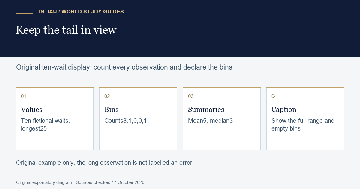
A display can be arithmetically correct yet invite a misleading conclusion. Ten fictional waiting times mostly sit between one and five minutes, with one value of twenty-five. This exercise asks you to preserve that long wait, state the bin boundaries and distinguish a typical observation from the arithmetic mean. It is a self-study display task, not evidence about an actual service.
Documentation boundary
NumPy’s histogram reference permits an explicit sequence of bin edges. All bins except the last exclude their right edge; the last includes it. The worked task supplies fixed equal-width edges and uses counts, avoiding an unstated density or bin-selection convention.
Write a display contract
The fictional minutes are one, one, two, two, three, three, four, four, five and twenty-five. Use five-minute bins spanning zero through twenty-five. Label the horizontal axis as waiting minutes and the vertical axis as observation count. Include the sample size ten. Start count bars from zero and preserve the empty middle bins. These choices make the long gap visible rather than compressing it out of the display.
| Bin in minutes | Count | Interpretation |
|---|---|---|
| 0 inclusive to5 exclusive | 8 | Main concentration |
| 5 inclusive to10 exclusive | 1 | The five-minute observation |
| 10 inclusive to15 exclusive | 0 | Empty bin retained |
| 15 inclusive to20 exclusive | 0 | Empty bin retained |
| 20 through25 inclusive | 1 | The long wait is visible |
Before running the answer, place each observation into a bin manually. Pay particular attention to five and twenty-five. Then predict the mean and median from the ordered list. The task is not to select whichever summary gives the most flattering impression; it is to explain what each summary says about this deliberately uneven example.
Check the counts and summaries
import numpy as np

values = [1, 1, 2, 2, 3, 3, 4, 4, 5, 25]
counts, edges = np.histogram(values, bins=[0, 5, 10, 15, 20, 25])
assert counts.tolist() == [8, 1, 0, 0, 1]
assert edges.tolist() == [0, 5, 10, 15, 20, 25]
assert sum(counts) == len(values) == 10
assert sum(values) / len(values) == 5
assert (sorted(values)[4] + sorted(values)[5]) / 2 == 3
without_tail = values[:-1]
assert sum(without_tail) == 25
assert round(sum(without_tail) / len(without_tail), 3) == 2.778
print("counts8,1,0,0,1; mean5; median3")
This snippet requires NumPy; the local author check used NumPy2.3.5 with Python3.12.14, while the linked stable reference was labelled2.5. The five bin counts are eight, one, zero, zero and one. They sum to ten, so every observation is accounted for. The total wait is fifty minutes, giving a mean of five. The two middle ordered values are both three, giving a median of three. A caption can report both values alongside the visible tail, rather than using one number to stand for the whole distribution.
Draw the histogram on paper or in a local plotting tool using the declared axes. The root publication diagram illustrates the study process, not a substitute measured service chart. If you use a charting library, check the displayed labels and full range against the table. A default plot with different edges may be legitimate, but it is a different display and should not be presented as the answer to this exact binning task.
Diagnose a misleading crop
A cropped chart ending at ten would omit the twenty-five-minute observation unless the omission was clearly declared. It could make the experience appear more concentrated than the full fixture supports. Do not silently remove the tail as an outlier merely because it looks unusual. The exercise supplies no evidence that the long wait is a recording error. A cleaning decision needs a reason beyond making a smoother picture.
For comparison only, removing that tail leaves nine observations totalling twenty-five minutes, with a mean of about2.778. Label this as a deliberately changed dataset, not as an improved estimate. The difference demonstrates the influence of the long value. It does not establish whether the original observation was wrong, nor does it justify excluding inconvenient measurements in another analysis.
Submit an honest caption
Your final caption should name the fictional quantity, the sample size, the bin rule, the mean and median, and the fact that the full tail remains visible. Explain why the empty bins matter: they separate the main concentration from the final observation. Include the count table so another learner can reconstruct the chart without relying only on its visual appearance.
As an extension, move the final observation from twenty-five to twenty-four. The final bin count stays one, but the mean changes to4.9 while the median stays three. This shows that a binned chart deliberately compresses detail. Keep the underlying values beside your display and avoid claiming that identical bin counts imply identical datasets. The task is complete when the values, table, summaries and caption tell a consistent story.
Questions for this exercise
Which bin includes the final right edge?
The NumPy convention includes the right edge in the final bin; the other bins exclude their right edge.
Must the long wait be deleted?
No. This fictional exercise provides no evidence that it is an error, so the full-range answer retains it.
Why show both mean and median?
Here they are five and three, describing different aspects of an uneven ten-observation fixture.
Official documentation
Explore the Courses overview or use Contact for general enquiries. This is an original INTIAU editorial self-study exercise; no qualification is awarded.
Related guides
View the study diagram